Great Fires: Chapter 2

[COMMITTEE NOTE: Most of the detailed GLO background, methodology and map interpretations have been relegated to Appendix D. I recently updated and re-formatted a 1992 report into Word that has fairly detailed descriptions of several sources of information listed in this chapter, as does my 1999 MAIS thesis, which is linked to an 11.8 mb. PDF file for easy reference. I will provide page numbers and links for these references at points in this chapter where I think they can provide additional, relevant, and/or otherwise complementary, information.]

CHAPTER 2.

METHODOLOGY

The basic premise of this thesis is to compare changing landscape patterns over time, in order to test the hypothesis that an elimination of Indian burning practices contributed to an increase in frequency and intensity of Oregon Coast Range forest fires. The primary formats used are maps and tables, to compare spatial and temporal patterns. Figures and text are used to illustrate and describe these patterns in context to the hypothesis and to consider such patterns at a finer, more local scale. Geographic Information Systems (GIS) software was used to create new maps and compare spatial and temporal patterns of Indian burning and catastrophic wildfire.

I used standard archival and anthropological research methods to obtain early surveys, maps, drawings, photographs, interviews, GIS inventories, eyewitness accounts and other sources of evidence that document fire history for the Oregon Coast Range. Focus was on spatial and temporal patterns of Indian burning across the landscape from 1491 until 1848, and corresponding patterns of catastrophic fire events from 1849 until 1951. Data were inventoried, tabulated, mapped and digitized as GIS layers (see Table 2.03) for comparison.

The research in this thesis was performed in accordance with the "method of multiple working hypotheses" first described by Chamberlin in 1890 (Chamberlin 1965): "the effort is to bring up into view every rational explanation of new phenomena, and to develop every tangible hypothesis respecting their cause and history". Two key features of this methodology are that research questions are answered based on the "weight of evidence", and research findings include the formal identification of additional "tangible" questions as they present themselves. Chapter 6 recommendations include several tangible questions developed through this research.

This chapter identifies study boundaries, types of information, and methods used to construct and compare GIS layers, maps and tables assembled to address the research of this thesis. It is composed of three parts. The first part describes principal exterior and subdivisional boundaries of the study area, including brief description of four research focal points, and provides references to detailed maps of these areas. Part two is a listing and general description of the types of information that were used to conduct research, and shows how data were organized into GIS layers, maps and tables for purposes of display and analysis. Part three defines and compares the three basic spatial scales used to display and compare the GIS fire and vegetation patterns that are the principal method of analysis and display for this study.

A. Research Boundaries and Focal Points

The Oregon Coast Range is bounded by the Pacific Ocean on the west, the Columbia River on the north, the Willamette and Umpqua rivers on the east, and the middle fork of the Coquille River on the south (Orr, et al.: 1992: 167). For purposes of this study, the Coast Range was divided into four subregions: labeled North, East, West, and South (see Map 1.01). The primary reasons for these divisions were to create a finer scale to display and consider research data, and because significant differences were found to exist between each of the subregions. Chapter 1 identified subregional differences in drainage patterns, topography, weather, and vegetation types. Chapters 3 and 4 will show that subregional differences also exist for precontact cultural landscape patterns, early historical land use patterns, and for catastrophic fire history patterns.

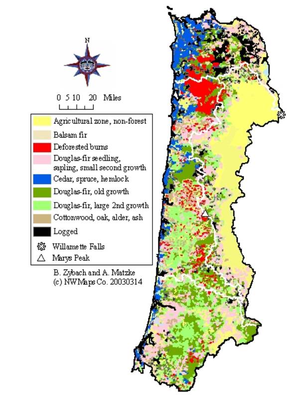
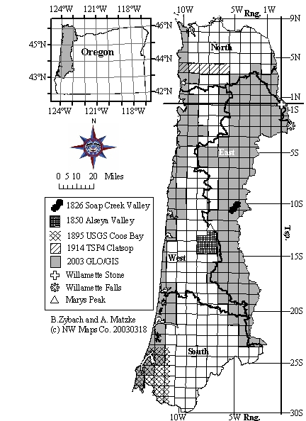
Map 2.01 is an index for the entire study. In addition to the four subregions, locations for various areas and landmarks will be in accordance with standard survey terminology: township, range, and section (see Appendix D), which are designated by the numbering grid shown on the map. Shaded townships show those areas that have been mapped from original land survey notes and converted to GIS layers by Oregon State University (OSU) researchers (Christy and Alvorsen 2003). Marys Peak and Willamette Falls will be used as reference points throughout this thesis, representing the highest peak in the Coast Range, and the abrupt change to tidewater taken by the Willamette River, nearby to the Willamette Stone survey marker (McArthur 1982: 798). The four focal points of each subregion are also shown: Tsp. 4 N., Clatsop County; Soap Creek Valley; "Alseya" Valley; and the Coos Bay Quadrangle.

Map 2.01 Oregon Coast Range study index.

1) North: Tsp. 4 N., Clatsop County

The northern subregion (“North” or “northern Coast Range”) follows the established Coast Range boundaries on the north (Columbia River), east (Willamette River), and west (Pacific Ocean). Its southern boundary is the southern watershed boundary of the Nehalem River and the northern watershed boundary of the Tualatin River. It is likely an important part of the fire history of the northern Coast Range that three of its boundaries are large expanses of water and, further, all of the borders are affected by daily tidal actions, seasonal flooding, and are known for their moist, foggy climates.

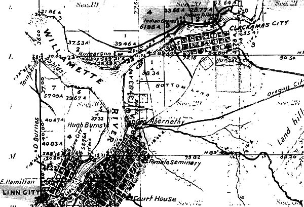
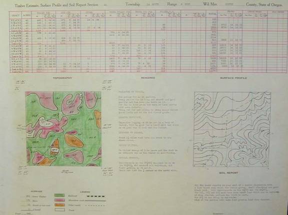
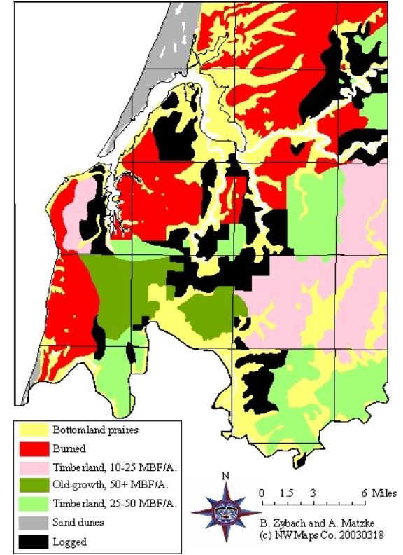
The focal point of research, done on a somewhat representative and much finer scale than the subregional patterns, is the entire 30-mile east-west length of Township (Tsp.) 4 N. (North of the Willamette Stone Baseline), as shown on Map 2.01. This focus was selected due entirely to the ready availability of an original 1913 timber cruise of the area. Both the date (pre-automobile) and the detail (see Map 4.02) worked very well for comparison to other historical maps (see Map 4.03). The maps were made available for extended study by Larry Fick (2003) and George Martin (2003) of Forest Grove Department of Oregon Department of Forestry (ODF). Tsp. 4 N. appears to be slightly smaller than five full Tsps. (180 square miles), because of the jagged Pacific Ocean western boundary; and appears to be about 110,000 acres in size.

2) East: Soap Creek Valley

The eastern subregion (“East” or “eastern Coast Range”) includes all of the Coast Range rivers flowing into the Willamette River. Its northern boundary is the northern watershed boundary of the Tualatin River; its eastern boundary is the Willamette and Umpqua rivers; the western boundary is the north-south ridgeline boundary that separate the eastward flowing rivers tributary to the Willamette, from the westward flowing rivers that empty directly into the Pacific Ocean (see Maps 1.02 and 1.03) of Coast Range rivers tributary to the Willamette; and its southern boundary is the northern watershed boundary of the Umpqua River. This is the driest and flattest of the four subregions.

The focal point of research for East is Soap Creek Valley (see Map 2.01), a 15,000 acre sub-basin, tributary to the Luckiamute River (see Map 3.03). One reason for selecting this area is that I had already performed a significant amount of related research in Soap Creek Valley in pursuit of my MAIS degree (Zybach 1999). Other reasons include its central location in the eastern Coast Range, the availability of local records, the somewhat typical nature of its general forest history as a small, east-facing, foothill valley, and the availability of GIS layers based on 1851-1910 GLO surveys (see Map 2.01; Christy & Alverson 2003; Map 3.04).

3) West: Alseya Valley

The western subregion (“West” or “western Coast Range”) includes all of the Coast Range rivers south of the Nehalem, west of the Willamette basin, and north of the Siuslaw that flow into the ocean (see Map 1.03). Its northern boundary is the southern watershed boundary of the Nehalem River; its eastern boundary is the north-south ridgeline divide from the Willamette River; its western boundary is the Pacific Ocean; and its southern boundary is the northern watershed boundary of the Siuslaw River. This subregion has the greatest percentage of Douglas-fir forestland and the longest stretch of coastal fogbelt forest of the four subregions.

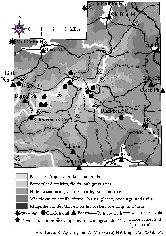
The focal point of research for West is Alsea (or "Alseya") Valley, a 90,000 acre sub-basin tributary to the Alsea River, to the immediate southwest of Marys Peak (see Map 2.01). This area was the focus of a paper I presented to the 5th annual Coquille Cultural Preservation Conference in 2003 (Zybach 2002). The principal map associated with the paper is Map 2.13. Most of the precontact map projections and early historical vegetation map patterns were developed with GLO survey data, recorded between 1853 and 1897 (see Appendix D).

4) South: Coos Bay Quadrangle

The southern subregion (“South” or “southern Coast Range”) is bounded on the north by the southern watershed boundaries of the Siuslaw and Willamette rivers (see Map 1.03). Its eastern boundary is the mainstem Umpqua River; its western boundary is the Pacific Ocean; and its southern boundary is the Middle Fork of the Coquille River (Orr et al. 1992). South is bounded by the Cascade Range to the east and the Klamath and Siskiyou Mountains to the south. It has greater amounts of black oak, tanoak, myrtle, and Port Orford whitecedar than the other three subregions combined.

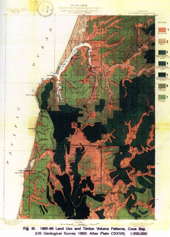
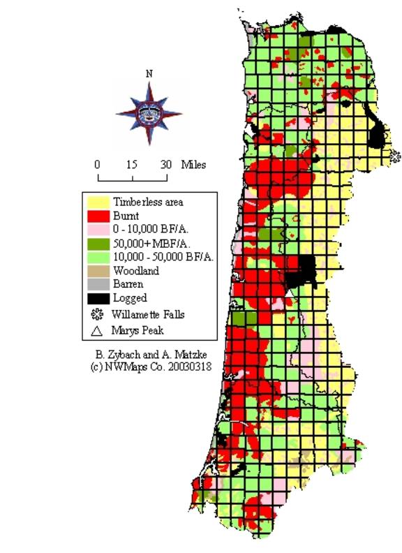
The focal point of research for South is that portion of the 1895-1896 USGS 30-minute quadrangle map (see Map 2.01; Map 2.06) to the north of the Middle Fork of the Coquille River and to the east of the Pacific Ocean. A principal reason for selecting this area is that I own the map in question, and helped participate with ODF to get the map digitized into GIS layers in 1995 (see Map 2.07). My familiarity with its contents, its age, quality of data, and ready access to a GIS version were other reasons this area was selected. An acreage estimate of the total land area of this focal point remains to be done.

B. Sources of Information

There were seven basic types of information used to complete this study: names on the landscape; persistent vegetation patterns (including tree rings); literature (principally historical and scientific); living memory (consultants, oral histories, and oral traditions); historical maps and surveys; aerial photographs; and digitized GIS (Geographic Information System) map layers. This section of the chapter provides examples and brief descriptions of each type, including representative examples of how they were used.

The value of different types of information varies significantly, depending on the time frame being researched, or the focus of a query. For precontact time, the most useful information came from paleoecological studies of pollen and tree rings; from archaeological and anthropological studies of local artifacts and native peoples; from historical forest maps; from consultations with experts; and from persistent patterns of native vegetation that can still be identified on aerial photographs and satellite imagery. For early historical time, from 1770 to 1850, the most valuable information was obtained from journalists and documentary artists. From 1851 to 1900, General Land Office survey notes and maps, and landscape drawings and photographs, provided the best methods to document the region's forest and fire history, and also provided the best method to predict precontact conditions. In 1900 the federal government began publishing the first of several reports on the forests of the Pacific Northwest, including those of the Oregon Coast Range that provided maps, photographs, tabular data, and detailed written descriptions (e.g., Leiberg 1900; Gannet 1902). In 1914, following the lead of the federal government, and in response to striking changes in property tax law, Oregon began producing detailed maps and reports through its own Department of Forestry (Elliot 1914) and the Timber Tax Division of the Department of Revenue (Zybach and Maeder 1996). Much agency work was based on the maps and logs of private timber cruisers, who created their own body of work from the late 1800s until the end of the study period (e.g., Bagley 1914). Other critical timeframes were the 1930s and the practical introduction of aerial photography, and the 1980s, with the practical beginnings of GIS.

1) Names on the landscape

A significant number of landscape features on the Coast Range provided strong clues and information regarding prehistoric cultural and ecological conditions important to this study. Indian nations, native food plants, wildlife habitat patterns, and past environmental conditions were often named and easily located through knowledge and records of such names. The most obvious example is the names of most Coast Range Rivers--including the Clatskanie, Coos, Yaquina, Nehalem, and many others (see Map 1.03), which clearly identify the Indian nations, and tribes that occupied those areas at the beginning of historical time. In a similar fashion, Oak Point, Onion Peak, Grass Mountain, Camas Valley, Peavine Ridge and the numerous Burnt and Bald peaks, ridges, and mountains provide additional information and insights (see Appendix B).

Coast Range landscape names related to native species, plant environments, and plant conditions are of particular interest to this study. The patterns of these names across the countryside and in correlation to prehistoric cultures proved to be good indicators of the relative importance of certain landscape features, the location of specific plant species, and the occurrence of past events. Named landscape features were also good focal points for additional research: Oak Point, for example, was named in 1810 and notes the furthest point west that oak trees were found along the Columbia River at that time. The same grove was documented by Lewis and Clark on March 26, 1806 and by Thompson on January 11, 1814. The name has since migrated across the river to Washington State, but it originally designated a grove located in Oregon on the northern edge of Fanny's Bottom, a flat bottomland prairie in Chinook country that took its name from nearby Fanny's Island, named by Clark for his sister, Frances (McArthur 1982: 551). Fanny's Bottom may have also been the location of a large Klaskani townsite, allowing these Athapaskan speakers a direct access to Columbia River trade routes otherwise controlled by Chinookans (see Map 3.01). Another example is Camas Valley, on the Middle Fork Coquille. This area had previously been named "Wheat Prairie" about 1850 by a group of "explorers" said to have noted "here and there were patches of wild wheat supposed to have been planted by Indians" (Connolly 1991: 7).

Appendix B is a listing of Coast Range landscape features named for native food plants (e.g., Salmonberry River and Fern Hill), native tree species (e.g., Cedar Creek and Yew Creek), native plant environments (e.g., Enchanted Prairie and Forest Peak), and native plant conditions (e.g., Deadwood Creek and Burnt Ridge). Names of towns and post offices are generally excluded as they are usually of more recent vintage and not always good indicators of local conditions: Forest Grove, for example, was named after a man's land claim, rather than a grove of forest trees (McArthur 1982: 283); Berry Creek was named after Thomas Berry rather than a local plant population (ibid.: 57); the community of Laurel wasn't named until 1879 (ibid.: 436); and the Meadow post office wasn't established until 1887 (ibid.: 487). Names were generally obtained from historical texts and maps and from two current Atlases (Benchmark Maps 1998; Pittmon Map Co. 1997). They are listed by county and legal description to establish provenance and distribution, and key names are located on several maps included in this study. Whenever possible, names were researched for authenticity (usually in McArthur 1982) before being listed or mapped.

2) Persistent vegetation patterns.

Persistent patterns of vegetation provide some of the most detailed information regarding precontact forest and fire history. Three basic sources of this type of data are pollens, tree rings, and documented populations of vascular plant perennials .Several native species of trees, shrubs, forbs, and grasses are useful for reconstructing precontact and early historical landscape patterns of vegetation. Trees (e.g., Douglas-fir, white oak, and Sitka spruce) are particularly valuable for such uses for at least four reasons: 1) they are long-lived and relatively pure stands of individual species often occur that are hundreds of years old, therefore the patterns of these stands can remain consistent from precontact time well into the current period of living memory; 2) they are usually the dominant form of vegetation in a stand, are readily identifiable from a distance (therefore providing consistency in interpretation from a variety of sources, including maps, drawings, landscaped photographs, and aerial photographs), and can usually be characterized by only one or two principal species (e.g., "a stand of Douglas-fir", or "a spruce-hemlock stand"); 3) following death, their remains, including snags, logs, and stumps, can persist dozens or hundreds of additional years, thereby providing opportunities for additional interpretation; and 4) annual and seasonal growth is recorded in "rings", which can be used to age stands (e.g., Impara 1997), measure relative variations in growth over time (e.g., Weyerhaeuser Company 1947), and interpret past climatic conditions (e.g., Fritts and Shao 1992). While shrubs (such as salmonberry and huckleberry), forbs (such as camas and brackenfern), and perennial grasses are not so reliable or versatile for interpretation as trees, they do form identifiable patterns across the landscape and can also persist in the same locations for decades or centuries (see Appendix D and Appendix H).

Pollen. A temporal test of long-term persistence is provided by fossil plant pollens, which can track change and migration of local plant species in an area over periods of thousands of years time. They provide a far more general and less reliable form of information provided by tree rings or documented vegetation patterns, but extend the record of fire and species composition much further into the past. Hansen conducted the first series of pollen studies in the Pacific Northwest, beginning in the late 1930s. Core drillings were made of peat deposits that had accumulated in relict bogs throughout the region. Many of these bogs dated to the last deglaciation, more than 12,000 years ago. Tree pollens preserved in the peat were counted and identified at specific intervals along the cores, showing the changes in local tree species assemblages through time (Hansen 1947). Although pollens are deposited and preserved chronologically, factors like gravitational pressure, floods, and long-term climate changes create problems with dating (Hansen 1945). Hansen helped resolve some of these problems by relying on volcanic ash deposits from Mount Mazama, Mount St. Helens, and the Three Sisters to date his western Oregon cores (Ibid.: XXX). His interpretations were then cross-referenced by a geologist (Allison (1946: 63-65) and an anthropologist (Cressman 1946: 43-51) to test the accuracy of his findings.

According to Hansen (1947: 84-86), lodgepole pine (shorepine) was the pioneer invader species in the northern part of the Willamette Valley after the most recent subsidence of Lake Allison, about 12,800 years before the present time (BP). By the time of European American immigration in the 1800s, lodgepole had been entirely eliminated from the valley; its decline and extirpation paralleled by the advent and persistence of white oak and increases in local Douglas-fir populations. Hemlock seems to never to have been prevalent in the valley since postglacial times, possibly because of the dry summers that characterized the region's climate during this period (CITE). The Willamette Valley pattern for lodgepole is the reverse of his analysis of coastal bogs covering "most or all of postglacial time" (Hansen 1944: 632), in which deposits of predominantly hemlock and Sitka spruce pollens are replaced over a 10,000 year or so period primarily with deposits from lodgepole. A radiocarbon-dated study of the ash and pumice profiles noted by Hansen was used to create a more specific time-line of his findings in 1964 (Hansen 1966:102). The following timeline for Oregon Coast Range postglacial forest and fire history, and climatic interpretations that can be drawn from it, is based on a discussion of the1964 radiocarbon-dated timeline with Hansen (1989: personal communication), after 25 years reflection:

12,800 BP to 8000 BP. A period of cooler, wetter time than the present, resulting in a coastal forest dominated by hemlock and spruce. People began to arrive in western Oregon from Asia during this time, although it may be that other people were already here.

8000 BP to 4000 BP. Hansen termed this period the "thermal maximum" because it was characterized by warmer and drier conditions, and included the apparent introduction of oak and the expansion of ponderosa pine populations in the Willamette Valley near the beginning of the period. Several ice age mega-faunas became extinct during this interval, a probable result of climate changes and/or human hunters. Coastal forest populations of Douglas-fir, lodgepole, and grand fir increased dramatically, corresponding to an apparent increase in the number and frequency of "holocaustic" fires and decreases in spruce and hemlock. Heusser (1960:184-185) referred to this period as the "Hypsithermal," which he defines as beginning and ending with a "mean annual temperature higher than at present," and which he dates at 8500 to 2500 BP Hansen was uncertain whether Pyne's (1982) observation that people bring "regularity and certainty" to a fire history had any bearing on the proliferation of Douglas-fir during this period, but didn't entirely discount the possibility. He also acknowledged the possibility that oak had been introduced into the Willamette Valley by people, but thought the same process may have been able to have been achieved by climate change and wildlife transport.

4000 BP to now (Heusser says 2500 BP to now). As the climate cooled to current temperatures, the end of the thermal maximum interval was followed by a fluctuating succession of Douglas-fir, spruce, lodgepole, grand fir, and hemlock forests to the general historical mix of shorepine, "fog belt" spruce and hemlock combinations, and inland even-aged stands of Douglas-fir and alder.

Although Hansen's research gives us information and insights into climate changes and basic forest sequence patterns, it provides few clues as to specific forest locations and structures. Additional inferences for developing that type of information must be derived from geological (slope, aspect, elevation), ecological (plant assemblages, soil types, landscape patterns), and anthropological (ethnobotany, cultural fire uses, archaeological findings) sources. Since 1989, Whitlock has done pollen studies for a small sub-basin of the Coast Range (Whitlock 1992), and tree ring (Impara 1995) and lake sediment (Long et al. 1998) studies have been performed in the same area; within a few miles of Hansen's 1942 Swamp Creek study. Otherwise, there remains very little paleoecological research performed on the Oregon Coast Range and all conclusions must be very general.

The value of isolated and localized pollen analysis and lake sediment interpretations for this study is marginal, except to provide broad climate, fuel, and fire backgrounds. However, tree rings and historical patterns of vegetation are key sources of information, particularly for late precontact and early historical time, from ca.1600 to ca.1850. Very little information of this nature exists in the Coast Range for the 1491 to 1600 period, and hardly any information all all has been discovered from before that time.

Tree rings. Tree-ring analysis dates back at least 400 years, when Da Vinci observed the relation of ring width to wet and dry years (Bennett 1948: 2). In the US, Keuchler completed an 1859 study that related oak tree ring widths to annual precipitation; however, the science of dendrochronology is said to have begun with the 1904 studies commenced by Douglass, of the University of Arizona (ibid.: 2). This methodology was initiated in the late 1930s in the Pacific Northwest (about the same time as Hansen's pollen studies), largely in an attempt to uncover evidence of cyclic precipitation patterns to predict drought (Graumlich 1987:19). Shinn (1977:92), for example, reproduces a 1937 "tree ring calendar" by Keen that charts tree-ring variations in eastern Oregon from 1268 to 1937. Graumlich (1987:25-26) also uses tree rings to analyze occurrences of droughts in the Pacific Northwest. Her findings of significant episodes during the late 1700s, the 1840s, the late 1860s, the 1920s, and the 1930s correspond to catastrophic forest fire events in the Coast Range during the same periods (see Chapter 4). In addition, a drought episode recorded for the time around 1680 could have contributed to wildfires that helped defined the parameters of later events. Further analysis of coastal tree rings would likely form a good test of this hypothesis.

Vegetation patterns. Patterns of tree species important to this study can be characterized as conifer or hardwood. Most Coast Range forestland is dominated by conifer trees, which are, for the most part, nearly pure stands of Douglas-fir (see Map 1.09). Other important species include a thin strip of shorepine that occurs along the western-most forested area of the coast; a belt of spruce-hemlock stands that dominate the coastal fogbelt to the immediate east of the shorepine strip; and stands of true fir, mostly grand and noble, that exist at higher elevations, such as Euchre Mountain and Marys Peak. Other conifer species, such as hemlock and Ponderosa pine, also exist in fairly pure stands, but they are scattered throughout the Range and typically constitute a minor part of the environment. Native species such as yew, redcedar, and chinquapin also occur throughout most of the Coast, but rarely create pure stands of any magnitude. These patterns of trees--large and small, living and dead--form the primary patterns of fuels that exist at the time of a forest wildfire.

3) Literature

Scientific and gray literature were researched for this study. Scientific literature, including studies of tree rings and pollens described in the previous section of this chapter, focused on disciplines related to studies of people, fire, and forest history specific to the Oregon Coast Range. Gray literature included newspaper and magazine articles, local histories, memoirs, and other published accounts of specific interest to this study.

Scientific studies of precontact and early historical people in the Oregon Coast Range usually fall under the headings of ethnography and archaeology. Archaeology is the science of reconstructing the history of people by studying the physical evidence they have left behind. Three basic methods are used in western Oregon; stratigraphic excavation, radiocarbon dating, and topological cross-dating (Aikens, 1984: 1). Analysis of artifacts from a site can show the types of animals eaten, species of wood used for fuels, approximate size of the local human population, and so on, for a given time and area. The location of specific sites is generally withheld from the public to discourage looting or other damage. Environmental changes can also be inferred from the analysis of such sites. Evidence from the Yaquina Head site, for instance, was used to support the possibility of a major coastal earthquake during the 1600s (Minor 1989:77). The primary problems with coastal archaeological sites in this study is that these populations largely depended on shellfish and marine mammals for much of their subsistence--commodities that were locally unavailable in inland valleys such the Willamette or Umpqua--and that many sites in excess of 4000 years of age may have been covered by rising seas caused by deglaciation (Aikens 1984:70), or by erosion (Minor et al., 1987:19). The principal value of ethnographic studies were the reports of interviews with living representatives of precontact tribes (see Appendix C). These are covered in more detail in the Living Memory section of this chapter. Other types of relevant scientific literature include forest ecology, fire ecology, and wildlife sciences, which form a minor part of this research, and which are covered in more detail in relevant portions of the thesis. Scientific literature related to Indian burning has increased in the past ten years (Williams 2003), but--other than the Willamette Valley--little of it is directly applicable to the remainder of the Coast Range (e.g., Boyd 1999b; Vale 2002). The same pattern holds true for Coast Range catastrophic fire history. With the exception of the Tillamook fires of 1933-1951, little research or attention has been paid to the other Great Fires of the Coast Range. Morris (1934b) and Pyne (1982) have described these fires, but Morris' article was written nearly 70 years ago, and Pyne's book does little more than paraphrase Morris. There is no literature that relates patterns of Indian burning in the Coast Range to subsequent patterns of forest wildfires.

Gray literature review involves historical studies, newspaper and magazine articles of current events, and primary documentation, such as memoirs, journals, diaries, and letters. For certain time periods and/or events, these forms of literature are the principal data used. Individual journals kept from 1788 to 1849 (see Table 2.01), for example, are the most complete and detailed records and eyewitness accounts that exist for early historical Indian burning practices in western Oregon. Table 2.01 shows the disparity in historical record-keeping chronology that exists in the Coast Range. Spanish, British, Russian, African, and American sea traders traveled up and down the Oregon Coast for several decades in the late 1700s, but had little information regarding inland areas. In the early 1800s, exploration of the Columbia River (northern Coast Range) increased dramatically, resulting in the establishment of Fort Astoria in 1810, and of Fort Vancouver in 1825. At that time (mid-1820s), overland explorations of the Oregon coast, and the Willamette, and Umpqua valleys began in earnest. By the late 1840s, most of the Coast Range was fairly well-known to informed residents and certain US government agencies. In all, it took about 75 years before most of the coastal rivers had been explored and mapped, resulting in a 75+ year history for the western Coast Range, a 50+ year history for the North, and about 25 years for the East and inland South. All of the journalists were white males, so a certain amount of demographic bias needs to be taken into account for these narratives.

Table 2.01 Early journalists of the Oregon Coast Range, 1788-1849

Name	Year(s)	N	E	W	S	Source
James Cook	1778			W
Robert Haswell	1788			W		Elliott 1928

W. R. Broughton	1792	N
Lewis and Clark	1805-06	N				Thwaites 1959
Gabriel Franchere	1811-12	N

David Douglas	1824-27	N	E		S	Douglas 1905; 1906
Alexander R. McLeod	1826-30		E	W	S	Davies 1961
Harrison Rogers	1828				S
Jedediah Smith	1828-29		E		S
John Work	1830-34		E		S	Scott 1923
David Lee	1835-45		E	W	S	Lee and Frost 1844
John Frost	1835-45	N		W		Pipes 1934

Charles Wilkes	1841	N				Wilkes 1845
George F. Emmons	1841		E		S
Brackenridge	1841		E		S	Sperlin 1931
Joel Palmer	1845		E		S	Palmer 1983
James Clyman	1846			W		Camp 1960
Theodore Talbot	1849		E	W		Haskin 1948
"Albert"	1849			W		Oregon Spectator, Sept. 9

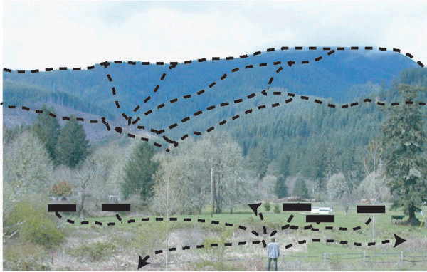
In addition to eyewitness journal descriptions of Coast Range peoples and forests, early cartographers, artists and draftsmen also made and kept records. Vancouver left a detailed set of maps behind his Northwest explorations, and Wilkes had an artist among the ranks of his 1841 expedition (see Fig. 3.01, Fig. 3.02, and Fig. 4.01). Fig. 2.01 shows an 1885 drawing of Marys Peak in the background of a house that still exists in the same location. Notice the smooth profile and lack of timber on the peak; a certain indicator of Indian burning, and a landscape condition that also exists to this time. Marys Peak is a well-known landmark clearly visible for dozens of miles from the surrounding countryside. It marked the entry to precontact and early historical "Alseyah Valley" by established foot and horse trails from the north and east (see Map 2.01). This drawing (Fagan 1885: 80) is of Felger's Mill (ibid.: 453, 513; Phinney 2000: 214), near present-day Philomath, to the northeast of Marys Peak. It clearly shows the grassy bald that characterized a significant number of Coast Range peaks at that time (Aldrich 1973). The Indian name for Marys Peak "is said to have been" Chintimini (McArthur 1982: 474). Nearby Grass Mountain was called Holgates Peak (Hathorn 1856a: 235), Prairie Peak called Blue Mountain (Gesner 1891b: 418), and Old Blue Mountain called Green Mountain (Collier 1891: 388) in early land surveys. Their Indian names are unknown.

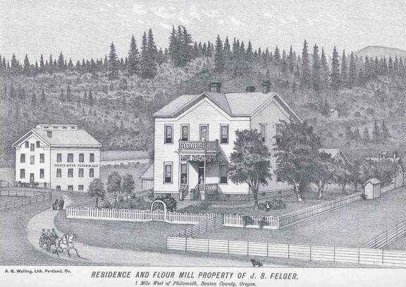
Fig. 2.01 Grassy bald on Marys Peak, 1885.

4) Living memory

Because the practices and events that are the focus of this study took place so long ago, eyewitness informants are limited, for the most part, to a decreasing number of older citizens who can recall or interpret only certain things about the most recent Tillamook fires. There are a few exceptions. Larry Fick (1988-2003: personal communications) and George Martin (1988-2003: personal communications) spent their careers studying and reforesting the Tillamook Burn and are intimately familiar with its history. Likewise, Jerry Phillips (1988-2003: personal communications) spent his career managing the Elliott State Forest that was carved out of the 1868 Coos Fire. All three were career employees of the Oregon Department of Forestry. Too, until his later years, Rex Wakefield (1976-1992) enjoyed a similar knowledge of the Yaquina Burn, both as a youngster performing "fern burning" activities to provide pasturage for his family's goat herd, and as Supervisor for the Siuslaw National Forest in the 1950s and 1960s. Numerous formal and informal communications with these four individuals over the past 15 and more years have helped to shape my understanding and knowledge of the Great Fires. Because Indian burning effectively ended in the Coast Range more than 150 years ago, there has been no living person during my lifetime with first-hand experience with these practices. What few accounts remain are in the forms of ethnographic interviews and brief observations by early historical journalists and residents.

Methods of obtaining living memory data include personal interviews, oral history research, and archival research. Personal interviews were limited primarily to the four people mentioned in the previous paragraph, and for the reasons mentioned. Focused oral histories that can be cross-referenced provide the most accurate and complete form of interview, but they require that the interviewee(s) be alive and willing. Additional value is gained by willingness to help, acuteness of memory, good verbal skills, and a skilled and prepared interviewer. Local informants are the best source of contemporary local history. The problem is that the first oral history recordings were not made until 1948, and I could not locate any from that time to the present that focused on the topics of this research. Further, I could see no purpose in initiating such a process, given the limited number of possible participants. However, published interviews that appeared in local histories, newspapers, magazines, radio scripts, and other formats were useful sources of information, as were ethnographic interviews performed with Coast Range Indians in the early 1900s (see Appendix C and Appendix F). The primary problem is with identifying the sources and locations of these interviews. County historical societies maintain WPA files, as do the University of Oregon library, the OSU Valley Library, and the Oregon State Historical Society Museum. A familiarity with local family names from pioneer times through World War II is essential to efficiently locating these documents.
Tape recorded interviews are also stored at the repositories listed above, as well as by the Forest History Society and OSU Archives, and they are often maintained by individual families as well.

Ethnographies are the formal studies of human cultures. Interviews made during the late 1800s and early 1900s by anthropologists with members and descendents of local families who inhabited the coast and Willamette Valley during late precontact and early historical time are of particular value. Individual members of the Alsi, Siuslaw, Coos, and Kalapuyan tribes were interviewed in this manner between 1910 and 1936 (e.g., Frachtenberg 1920, Jacobs 1936). One or more Yakonans may also have been recorded in 1884 (Minor 1989: p.3). Although concerned with lands east of the Cascade Range in Oregon, Shinn's (1977:23-28) analysis of Native American myths about fire use demonstrates several methods by which ethnographic data can be interpreted. Fagan's (1885:320-323) legend of romance involving Alsea, Klickitat, and "Drift Creek Indians", although not an ethnography, contains information of this sort that might be worth further study. Fig. 2.02 shows members of the Siletz tribe in a mixture of local, European, and Plains Indian clothing and decorative styles in 1924, attending the "Last Official Indian Ceremonial Ever Held in North Lincoln" (E. Nabut 1951: 105), a few miles from the present location of Chinook winds Casino. These people were descendents of Salish and Yakonan tribes that had been assimilated into the Siletz Indian Reservation, beginning in 1856 (Kent 1982). It is unlikely that nay of these people had clear recollection of precontact time. Most ethnographic interviews with Coast Range Indians were made between 1910 and 1936 and involved members of the Siletz or Grand Ronde reservations.

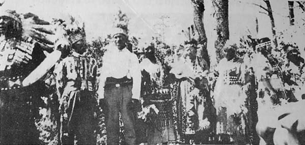
Fig. 2.02 Sources of living memory

5) Aerial photographs

Aerial photography was implemented in the 1920s by such organizations as the USDA Forest Service, the Oregon State Highway Commission, and the Soil Conservation Service. A good inventory of aerial photographs taken in Oregon before the summer of 1937 was assembled by the WPA (Bennett and Stanbery, 1937). After World War II, the availability of military aircraft and sophisticated photographic equipment and techniques developed during the war led to significant improvements in image quality and flight frequency. The University of Oregon has the most complete collection of aerials available in Oregon, but businesses such as W.A.C. (Western Aerial Contractors) in Eugene and organizations such as the Forest Service maintain extensive collections that allow for the purchase and/or use of individual "site-and time-specific" sequences.

Aerial photographs are, in effect, highly detailed and time-specific maps of landscape patterns. Before aerial photography came into widespread use in the 1930s, people had to use maps or visit scenic vistas to consider landscape-scale patterns of vegetation and human constructs. Because aerial photography didn't exist during the time of Indian burning or, in a practical sense, prior to the 1933 Tillamook Fire, its use in this thesis is principally for interpretive (rather than documentary) puposes. The exception is the Tillamook fires of 1933-1951 which have been extensively photographed, otherwise documented, mapped and analyzed over the course of the last 70 years.

Aerial photographs were used extensively over the course of this research, particularly photos taken between 1939 (e.g., Zybach and Badzinski 1998) and 1966 (e.g., Fig. D.01). Fig. 2.03 is an aerial photograph of the town of Alsea, Oregon, taken on June 29, 1948. The juncture of the North Fork and South Fork of the Alsea River can be seen near the bottom of the photo. General Land Office (GLO) subdivision and Donation Land Claim (DLC) boundary lines dating to the early 1850s are clearly apparent as the straight courses of roads, fencelines, crop borders, and logging boundaries a century later. Fenced and plowed bottomland prairies, meadows, ridgeline trails, hillside scatterings, and other pre-contact landscape patterns can also be easily discerned. A principal difference between Indian and white cultural patterns, including firewood gathering and broadcast burning patterns, and as evidenced by this photo, is the imposition of straight lines on the landscape.

Today (2003) the bottomlands are still dominated by the town of Alsea--descended from the "Alseya Settlement" of 1855 (McArthur 1982: 12-13), in turn descended from the Alsi Indian community of Ts !Iphaha) (Drucker 1933: 82)--at the juncture of the North and South forks of the Alsea River, and the remainder consists largely of numerous family-owned farms and ranches. Surrounding uplands are heavily forested with a variety of hardwoods and conifers, particularly Douglas-fir, which forms about 90% of the population and volume of trees in the area (Bagley 1915; Munger 1916)

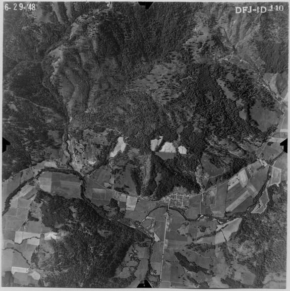
Fig. 2.03 Aerial photograph of Alsea, Benton County, Oregon, 1948 (Knight Library collection).

6) Historical maps and surveys

Three types of historical maps proved particularly useful to this research: original land surveys, local and county timber cruises, and statewide vegetation types. Other types of maps, including USGS quadrangle maps, property tax lot maps, land ownerships maps, and highway maps, also proved helpful, but did not contain the types of data that could be readily used to represent burning and wildfire patterns. Also, all of the GLO data (1851-1940), a good number of timber cruises (1913-1928), and three pre-aerial photo vegetation type maps (1900-1936) fell within the range of the 1849-1951 catastrophic fire history period.

GLO surveys completed throughout western Oregon between 1851 and 1910 provide an exceptional source of information for documenting the transition of environmental conditions from traditional Indian land management practices to introduced European practices (see Appendix D). Although these surveys were performed during the early 1850s and after, they can also be used to make reasonable estimates of environmental conditions at the time of contact, or even before (Zybach 2002). GLO land survey records have been long accepted as useful measures of past environmental conditions (Whitney and DeCant 2001: 147). These records have specific advantages over other early historical sources of information in being a definite sampling of vegetation, written on location, and in accordance to a predetermined plan (Bourdo 1956: 755).

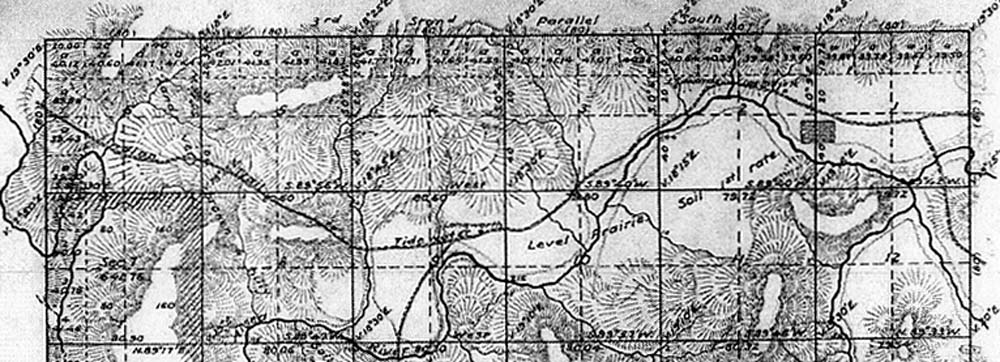
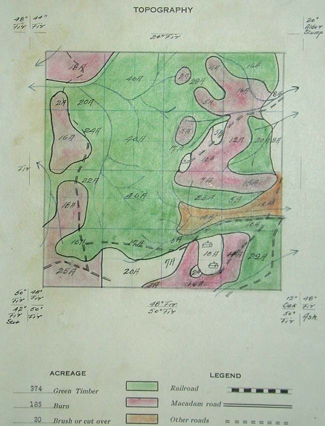
GLO survey notes and maps document environmental conditions systematically measured for the entire western US and a large portion of the eastern US from the late 1700s to the present. Original land surveys for western Oregon, including the Coast Range, were completed between 1850 and 1910 (Stewart 1935: 72-73). This voluminous source of data includes detailed information that is both quantitative and qualitative; is arranged in precise spatial components at a relatively fine scale; reflects a critical period of time in which American Indian resource management practices were dramatically altered by European American immigration and land appropriation; and was--significantly--gathered by a large number of surveyors operating under a single set of specific instructions (Bourdo 1956; Schulte and Mladenoff 2001). Fig. 2.04 is a page from the Benton County Surveyor's Office that was typewritten, possibly in the 1930s, from handwritten field notes. The subsequent colored notations were used to construct maps and GIS layers for this study. Several of these excerpts have been indexed in Appendix D. The blue marks show the exact distance and compass bearing from an established survey point that the surveyor enters a distinct vegetation type, such as a "bottom" or "thicket" (see table 3.03). The pink highlights show precontact cultural artifacts, such as prairies, Indian trails, and oak groves, and early historical artifacts, including Indian trails and David Fudge's house. The red ink and cross-hatchings mark the great distance--600 links ("lks") equal about forty feet--between bearing trees. This corner must have been within a "scattering" or savannah environment for oak and open canopy to be present. Further, the (probably) Douglas-fir trees were only 36 inches in diameter, making them fairly young second-growth trees that had probably been seedlings sometime after 1790, while the slower-growing oak were probably around 120 to 240 years of age. None of these trees were likely living before 1600. It is possible that first the oak, and then the Douglas-fir, encroached on what had once been an open field.

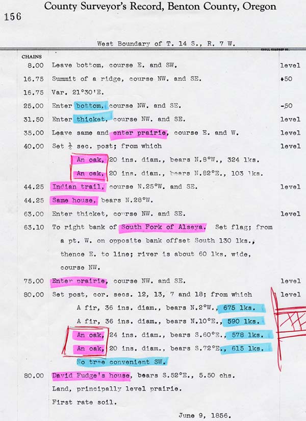
Fig. 2.04 Tsp. 14S., Rng. 7 W. annotated GLO field notes, 1856

GLO surveys began with the establishment of initial points ("meridians"), located for practical geographic reasons and recorded by astronomical observations. Thirty-five meridians were established in the continental US (Stewart 1935: 74). The initial point for Oregon Territory (then including Washington and Idaho), the "Willamette Meridian", was determined on June 4, 1851 (McArthur 1982: 798), in the West Hills above Portland. The location, later marked with the "Willamette Stone" (see Map 2.01), was selected on the basis of visibility, "that the Indians were friendly on either side of the line for some distance north and south" (Burnham 1952: 229), and because the east-west Base Line of the survey intersected the Columbia River in only one place.

Map 2.01 locates and names each of the six-mile square (36 square mile) townships in this study (Moore 1851: 227-230), relative to their position in the Coast Range. Beginning at the Willamette Stone, a north-south "meridian" and an east-west "baseline" serve as the beginning to a succession of six-mile wide tiers. Each east-west tier (also called "Township" and written as "Tsp." or "T.") is numbered consecutively north ("N.") or south ("S."), and each north-south tier (called "Range" and written as "Rng." or "R.") is numbered consecutively east ("E.") or west ("W."). The intersection of numbered township and range tiers form square townships designated by this numbering system. For example, the township containing Marys Peak (Fig. 2.01) is named Tsp. 12 S., Rng. 7 W. (or, T. 12 S., R. 7 W.) and can be located by counting 12 tiers south and seven tiers west of the Willamette Stone. Every surveyed township in Oregon and Washington is located and named in the same manner and commencing from the same starting point (Stewart 1935: 74). Most historical maps, including almost all timber cruises and vegetation type maps, and all current landownership boundaries and tax lot maps, are based on these lines. Before 1851, these lines were absent from the environment. Since that time they have served as an exacting index to specific trees, points, locations and cultural artifacts at specific days in time.

Map 2.02 shows the pattern of 36 square mile "sections" ("Sec." or "S.") created when surveyors subdivided a township. Table 2.02 lists the names of the surveyors that completed this map and others in the "Alseya Valley" area (see Map 2.13). The numbering is always the same--beginning in the NE corner with Sec. 1, continuing west to Sec. 6, then south one mile to Sec. 7, proceeding east through Sec. 12, and then repeating the sequence two more times, continuing to number consecutively, until Sec. 36 is reached in the SE corner of the township (Moore 1851: 229). If original land claims (called a "Donation Land Claim" or "DLC") or portions of DLCs are contained within the township, they are also numbered consecutively, beginning with the number 37, so as to not confuse them with section numbers. For example, the DLC of Basil Longworth, (Longworth 1972), No. 37, is contained in T. 14 S., R. 8 S., Secs. 9 and 10 (Hathorn 1856c: 491-493). When a land claim straddled more than one township, it was given separate numbers for each township. Squire Rycraft (Fagan 1885: 525-526), for example, was given DLC No. 45 for the 94 acres he claimed in T. 14 S., R. 8 W., and No. 40 for the remaining 66 acres of his claim to the east, in T. 14 S., R. 7 W (Hathorn 1856c: 496-497). Boundaries of Rycraft's 1856 survey are still readily apparent today, as evidenced by aerial photography (Fig. 2.03).

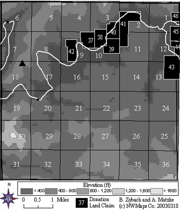
Map 2.02 Tsp. 14 S., Rng. 8 W. GLO subdivision and DLC survey index.

Table 2.02 lists the names of the men who conducted the original GLO land surveys in "Alseya Valley", the years and times of year they conducted their surveys, and the locations they described and mapped. It also indicates whether Indian foot or horse trails were noted, and when and where forest fires had occurred. In common with the earliest Coast Range journalists (1788-1849) and the Valley's original land claimants (see Map 2.02), all of the surveyors were white males. In July 1856, Dennis Hathorn surveyed each of the 15 Donation Land Claims (DLCs) that had been established in the Valley during the previous four years (Hathorn 1856c). Eight of the claims were for 160 acres each (1/4 section), and seven of the claims were for 320 acres (1/2 section). The larger claims indicate married couples. All of the claims were established along the mainstem Alsea River, along the main foot and horse trails from the Willamette Valley to tideland, on the best 2,500 acres of bottomland prairie in Alseya Valley (see Fig. 2.04, Map 2.12). By law, no Indians, Blacks, or Chinese were allowed to make or purchase land claims (Carey 1971: 253).

Table 2.02 Original GLO surveyors of Alseya Valley, 1853-1897.

Surveyor	Dates	Townships	Burns	Trails
Webster, Kimball	Oct.-Dec., 1853	14-7	X	X
Gordon & Preston	Sept., 1854	13-7	X
Hathorn, Dennis	June-July, 1856	13-7; 13-8; 14-7; 14-8	X	X

Mercer, George	Aug., 1865	13-7;	X
Dick, J. M.	Aug., 1873	13-8; 14-8	X
Mercer, George	Jan., 1878	14-7; 15-7	X	X

Gesner, Alonzo	May-July, 1891	14-7; 14-8; 15-7; 15-8	X	X
Collier, Charles	Sept.-Oct., 1891	13-7; 13-8	X	X
Collier, Charles	Feb., 1892	13-7	X
Collier, Charles	Apr.-May, 1893	14-7; 15-7	X	X
Sharp, Edward	July, 1896	15-7	X
Sharp, Edward	Jun.-Sept., 1897	13-8; 15-7	X	X

Surveyors described native plants in terms of species, general locations, and plant mosaic types. Vegetation types were also described in reference to land and property developments and often noted as they were encountered along GLO survey lines, DLC property lines, and riparian intersections. Bearing trees (Moore 1855: 8-9) were precisely located and listed by species and diameter in relation to the mosaics (e.g., Zybach 1999: 275-292); typically six or more trees per running mile, with a minimum of eight trees per forested section, and often more than eight for sections adjacent to double corners (Moore 1855: 12) or containing DLCs or riverine meanders (ibid.: 14). This process allows us to compare the measures and observations of individual surveyors and better evaluate our estimates of past environmental conditions. Surveyors regularly noted specific types and species of plants and whether forest fires had entered the area, or not. Collier gave this general description of Tsp. 14 S., Rng. 7 W. (approximately 36 square miles; or about 23,000 acres) in May, 1893, for example:

In addition to property lines, bearing trees, and vegetation patterns, GLO maps and survey notes contain a significant amount of information about cultural artifacts and developments. Map 2.03, for example, clearly shows the location of an Indian village and burial ground a few miles northeast of Willamette Falls. Map 2.03 is a good representation of the type of subdivision map that was developed from GLO field surveys. A second type of map for property owners, the DLC plat map (see Map D.02), was also produced at the same scale as the subdivision maps.

Map 2.03 Clackamas Indian village and burial ground, 1856.

GLO surveyors were specifically instructed to note cultural "improvements" to the environment, including "Indian towns and wigwams", and "natural curiosities", including "all ancient works of art, such as mounds, fortifications, embankments, ditches, or objects of like nature" (Moore 1855: 17-18). They were probably not trained to recognize such localized features as elk pits, peeled trees, or rock ovens. Fig. 2.03 illustrates lasting changes brought to Alseya Valley landscape patterns by white settlement and GLO surveys. Beginning with the establishment of DLC boundaries, native plant populations were soon limited and infiltrated by the plantations and structures of the new settlers. Surveyors duly noted and mapped fields, orchards, gardens, wagon roads, ditches, a bridge, a walk log, fences, barns, houses, an outhouse, a school house, a post office, and an old flume to "In man!s sawmill" in Tsp. 14 S. Rng. 7 W. (Fagan 1885: 500; Collier 1893: 178). As might be expected, more of these structural and vegetational changes are indicated in the GLO records from the 1890s than the 1850s, as the Valley became more heavily populated with immigrant farmers, ranchers, loggers, sawmill workers and their families.

This study demonstrates the potential of GLO maps and survey notes to make good estimates of precontact land use patterns and resource management practices. The detailed mapping of Indian canoe routes, foot and horse trail networks, homesites, and campsites in relation to managed fruit and nut orchards, berry patches, and extensive fields of root and grain crops cannot be duplicated by any other source of information. The location and timing of daily, seasonal, and annual practices of burning, tilling, and harvesting that took place in pre-contact times can be easily and reasonably inferred from these records. The precise location of individual trees and possible elk-fall pits provides exacting details of how and where people hunted, where they shaded themselves from the sun, and when they met to gather nuts or firewood. The great diversity and ready access of managed environments, including grassy prairies, oak groves, meadows, brakes, balds and berry patches provide strong insights into the lives of people and cultures that no longer exist. This combination of detailed records and reasoned insights are just as significant for considering pre-contact wildlife populations, habitat patterns, and food sources.

The other types of historical maps used extensively in this research are timber cruises and vegetation type maps, typified by Map 2.04 (Bagley 1915) and Map 2.05 (Peterson 1993: 12), both produced within a year or two of each other. The timber cruise map covers a single, 640-acre section of property. Each section is divided into four square "quarter secs" of about 160-acres each, called NE, NW, SW, and SE. Each quarter sec is also quartered, and also designated NE, NW. SW. and SE, but these "1/4 of a 1/4 secs" are 40-acres in size. Therefore, the NW 1/4 of the NW 1/4 of this section would be a square 40-acre pieces of land on the extreme northwest corner of the map. We can then go to the tally sheet and find the same location, where precise tree species, general diameters, and reasonably estimated volumes of each species are located. The maps provide polygon shapes that couldn't be shown on GLO maps. Typed and signed notes regarding timber markets, fire hazards, etc., also add details. These are the most detailed and exacting patterning of forest fires that predates aerial photography. Unfortunately, timber cruises of this quality do not cover all of the forested lands in western Oregon, and existing cruises are of a highly uneven quality.

Map 2.04 Tsp. 14 S., Rng. 8 W., Sec. 22 timber cruise, 1915.

Oregon's entire pattern of wildfires were mapped for Oregon State Forester F. A. Elliott in 1914 (Peterson 1994: 12). This map was prepared in advance of the 1918, 1933, 1939, and 1945 Tillamook Fires and clearly depicts over half of the Coast Range (south to the middle fork of the Coquille River) as “Burned & Restocked”, “Burned & Not Restocked”, “Brush”, and “Prairie”. There is also a large burned area around Tillamook Bay, possibly a result of the 1902 fire, that may have served as a partial buffer for the Tillamook Bay community against later events in 1910 to 1951. The boundaries of the Yaquina, Coos, and Nestucca fires of ca. 1849 to 1868 are clearly depicted, although of varying quality of detail. This statewide map has several advantages over the timber cruise map: it covers the entire region at a similar point in time (probably a six-month to six-year range of time the information was gathered before the map was printed), it was all composed of the same, uniform vegetation types, and it was available to the public. The principal disadvantages are that it has little practical value for land managers used to working in 40-acre increments, it contained far less information, and of far more general scale, and it was generally too bulky for field work. For purposes of this study, the 1914 Elliott Map also had value because it had been converted to a GIS coverage (ibid.: 12).

Map 2.05 Oregon State Forester's Map, 1914 (Photo by B. Zybach 1988).

7) GIS layers

This study used existing computerized Geographic Information System (GIS) map files to help construct new maps (see Table 2.03). Map files are called layers or coverages and can be in the form of points, lines, text, or polygons. Map information is stored in relational databases that are georeferenced: that is, they are created in precise relationship to their relative position on the surface of the earth in terms of longitude, latitude, and elevation. In this manner, individual coverages can be "layered" on one another with assurance that the data is displayed in accurate spatial relationships. For example, a point representing the center of the City of Corvallis might be used to locate the city's name in text; a polygon is layered over the point and text that represents the city's corporate boundaries; a line is layered over the polygon that represents Highway 99 W: viewed together, we would have a labeled map of Corvallis' city limits, showing where Highway 99 enters, passes through, and leaves town. Other points, lines, polygons and labels could be added to show and identify streets, blocks, creeks, property lines, etc., as desired.

Table 2.03 Sources and descriptions of GIS layers used for this study.

map	Filename	New Name*	Source-contribution	Type	Description
2.12, 4.12, 4.13, D.01	basin67_geo	6th_7th_Fields	CLAMS	Coverage	Sixth and Seventh Field Hydrologic Units for the CLAMS Area
3.05, 4.01, 4.08	east_bound2	East_boundary	new - CLAMS (basins) and ESRI (rivers)	Coverage	Outlines eastern Coast Range subregion boundary
1.01, 1.09, 2.01, 6.01, E.01	entire_bound2	Coast_Range_N_E_W_S	new - CLAMS (basins) and ESRI (rivers)	Coverage	Outlines complete study area and four N/E/W/S subregions
3.01	nations21	Indian_Nations_1775	new - CLAMS (basins) and ESRI (rivers)	Coverage	Outlines approximate Indian nation boundaries, ca. 1775
none	huc250k	USGS_Subbasins	USGS	Coverage	1:250,000-scale Hydrologic Units of the United States
3.02, 4.01, 4.04	north_bound2	North_boundary	new - CLAMS (basins) and ESRI (rivers)	Coverage	Outlines northern zone
1.01, 2.01	or_boundary	Oregon_boundary	ESRI - conus_states.shp	Coverage	Outlines state of Oregon boundary
1.03, 2.01, 2.09	outer_bound2	Coast_Range_1_boundary	new - CLAMS (basins) and ESRI (rivers)	Coverage	Outlines complete study area. Internal zones are not delineated
3.07, 4.01, 4.15	south_bound6	South_boundary	new - CLAMS (basins) and ESRI (rivers)	Coverage	Outlines southern zone
3.06, 4.01, 4.09	west_bound	West_boundary	new - CLAMS (basins) and ESRI (rivers)	Coverage	Outlines western zone
2.10, 2.14, 2.15, 3.02, 3.06, 3.07, 4.01, 4.03, 4.04, 4.08, 4.09, 4.11, 4.13, 4.14, 4.15, 6.02, E.03, f.01	bvbh1936	1936_PNW_Veg	ICBEMP-BLM	Coverage	1936 historical vegetation patterns for Oregon and Washington
4.03, E.01, E.02, E.03	fire1850	Teensma_1850	BLM	Coverage	Western Oregon Fire History, c 1850
4.03, E.01, E.02, E.03	fire1890	Teensma_1890	BLM	Coverage	Western Oregon Fire History, c 1890
4.03, E.01, E.02, E.03	fire1920	Teensma_1920	BLM	Coverage	Western Oregon Fire History, c 1920
4.03, E.01, E.02, E.03	fire1940	Teensma_1940	BLM	Coverage	Western Oregon Fire History, c 1940
6.01	ownership	1993_Landowners	SSCGIS	Coverage	1993 land ownership in Oregon
2.08, 2.14, 2.15, 4.01, 4.03, 4.04, 4.08, 4.09, 4.11, 4.14, 4.15, E.03	q100_veg1900	1900_USDI_Veg	BLM	Coverage	1900 historical vegetation patterns of Oregon
1.09	stateveg	1988_OR_Veg	ONHP	Coverage	1988 vegetation of Oregon
4.07	strands93	Soap_Cr_forest_ages	COF	Coverage	Cultural age classes for a piece of the Willamette Valley.
2.09, 2.14, 2.15, 3.02, 3.06, 3.07, 4.01, 4.03, 4.04, 4.08, 4.09, 4.11, 4.13, 4.14, 4.15, 6.02, E.03	timber	1914_ODF_Veg	SSCGIS	Coverage	1914 historic timber coverage for Oregon
2.01, 2.07, 2.08, 2.11, 2.14, 3.04, 4.03, 4.11, 4.14, 6.02	townrng	OR_Tsp_&_Rng	SSCGIS	Coverage	Township and range lines for Oregon
1.02, 1.03, 2.02, 2.11, 2.12, 2.14, 2.15, 3.02, 3.05, 3.06, 3.07, 4.12, 6.02, D.01	bob_elev_f	Elevation_250,000	USGS	Grid	1:250,000 (3-arc second or 100-meter) DEM of Oregon
1.02, 1.04, 2.12, 3.01	bob_hlsd	Elevation_new	new-USGS	Grid	1:250,000 (3-arc second or 100-meter) hillshade of Oregon
1.04	bob_ppt_f	Rainfall_annual	SCAS PRISM - us_ppt14.asc	Grid	100-meter annual precipitation in Oregon
2.01	alseya_sections.shp	Alseya_sections	OR GISBenton County GIS - sectionlines.shp	Shapefile	Sectionlines for the Alseya Valley
2.11, 2.12, 2.14, 4.11, 4.12, 4.13, 6.02, D.01, E.02	alseya2.shp	Alseya_boundary_1	new-digitzied and SSCGIS (township and range)	Shapefile	Boundary of the Alseya Valley
4.12, 4.13	alseyatrails_box2.shp	Alseya_boundary_2	new-digitzied and SSCGIS (township and range)	Shapefile	Boundary of the extended Alseya Valley
2.01	clatsop1914_boundary.shp	Clatsop_Tsp_4N	new-digitzied and SSCGIS (township and range)	Shapefile	Boundary of specific townships to delineate a 1914 Clatsop area
E.03	coast16_bound2.shp	Ocean_GLO_GIS	new-ONHP (coastal GLO)	Shapefile	Boundary of the coastal GLO
2.07, 4.14	cbay_box8.shp	1895_Coos_Bay_Quad	new-ODF (1895 veg Coos)	Shapefile	Boundary of the Coos Bay area
1.02, 1.03, 1.04, 1.09, 2.01, 2.08, 2.10	bob_clip.shp	bound_enitre_mask.shp	new - CLAMS (basins) and ESRI (rivers)	Shapefile	Outlines complete study area and delineates 4 zones. Used as a mask.
2.01	GLO2003_boundary.shp	bound_GLO2003.shp	new - CLAMS (basins) and ESRI (rivers)	Shapefile	Boundary of 2003 GLO
2.01, 3.04	soap_creek.shp	bound_soapcreek.shp	new-digitzied and SSCGIS (township and range)	Shapefile	Boundary of 1826 Soap Creek Valley (estimate)
2.14, 6.02	glo1850_clip1.shp	clip_glo1850.shp	new-digitized and USGS (DEM)	Shapefile	Sub-boundary of 1850 GLO
2.14, 6.02	pnw1936_clip1.shp	clip_pnw1936.shp	new-digitized and ICBEMP (1936 veg historic)	Shapefile	Sub-boundary of 1936 PNW historical vegetation
2.02, 2.11, 2.12, D.01	bob_elev_ctour.shp	cntr_elev_ft.shp	new-generated and USGS (DEM)	Shapefile	Countour of DEM
3.02, 3.06, 3.07, 4.01, 4.04, 4.09, 4.13, 4.15, E.03	coast16.shp	coast16.shp	ONHP	Shapefile	Historic vegetation of the Oregon Coast
1.03, 2.09, E.01	conus_counties.shp	conus_counties.shp	ESRI	Shapefile	County boundaries of the US
1.03, 1.04, 3.01, 3.02, 3.05	conus_lakes.shp	conus_lakes.shp	ESRI	Shapefile	Lakes of the US
2.01, 2.07, 4.01, 4.14, 4.15	coos1895.shp	coos1895.shp	ODF	Shapefile	1895 Coos Bay historic vegetation
2.02, 2.11	donationlandclaims.shp	donationlandclaims.shp	OR GIS BC	Shapefile	Donation land claims in Benton County
2.11	point_alseacity.shp	point_alsea.shp	new-latitude/longitude	Shapefile	Location of Alsea, OR
2.11, 4.12, 4.13, D.01	alseya_trails2.shp	point_alseatrails1.shp	new-latitude/longitude	Shapefile	Location of features in Alseya Valley
2.12	alsea_trails3.shp	point_alseatrails2.shp	new-latitude/longitude	Shapefile	Location of features in Alseya Valley
1.04	city_test.shp	Coast_Range_Cities..shp	new-latitude/longitude	Shapefile	Location of cities in Western Oregon
4.12	point_klickitat.shp	Klickitat_Ridge..shp	new-latitude/longitude	Shapefile	Location of Klickitat Ridge
1.04	city_ppt.shp	Coast_Range_Stations.shp	new-latitude/longitude	Shapefile	Location of precipitation stations in Western Oregon
1.02, 1.03, 1.04, 1.09, 2.01, 2.08, 2.09, 2.10, 3.01, 3.02, 3.05, 3.06, 4.01, 4.04, 4.08, 4.09	twofeatures.shp	Marys_Peak..shp	new-latitude/longitude	Shapefile	Location of Willamette falls and Mary's Peak
1.02	willamette	Willamette_River..shp	new-NRCS (rivers)	Shapefile	Willamette River
1.03	major_rivers5	Columbia_River..shp	new-NRCS (rivers)	Shapefile	Willamette and Columbia Rivers
1.03, 3.01, 4.12, 4.13	bob_rivers10.shp	Alseya_Rivers..shp	new-ESRI (rivers)	Shapefile	Rivers in Alseya Valley
1.04, 2.02, 2.11, 2.12, 2.14, 3.02, 3.05, 3.06, 3.07, 4.03, 4.04, 4.08, 4.09, 4.11, 4.15, 6.02, D.01, E.01, E.02	bob_rivers7.shp	Coast_Range_Rivers..shp	new-ESRI (rivers)	Shapefile	Rivers in Western Oregon
2.02, 2.11, 2.15, 3.04, 4.07	sectionlines.shp	Benton_Sections..shp	OR GIS BC	Shapefile	Section lines in Benton County, Oregon
3.05, 4.08	east_trails.shp	East_Indian_Trailst.shp	new - CLAMS (basins)	Shapefile	Major trails network in the eastern zone. Created from CLAMS sixth/seventh field hydrologic units.
3.02, 4.04	north_trails.shp	North_Indian_Trails..shp	new - CLAMS (basins)	Shapefile	Major trails network in the northern zone. Created from CLAMS sixth/seventh field hydrologic units.
2.12, 4.12, 4.13, D.01	primarytrails.shp	Alsea_Indian_Trails..shp	new - CLAMS (basins)	Shapefile	Major trails network in the extended alseya valley area. Created from CLAMS sixth/seventh field hydrologic units.
3.07, 4.15	south_trails.shp	South_Indian_Trails..shp	new - CLAMS (basins)	Shapefile	Major trails network in the southern zone. Created from CLAMS sixth/seventh field hydrologic units.
2.12, 3.06, 4.09, 4.12, 4.12, D.01	west_trails.shp	West_Indian_Trails..shp	new - CLAMS (basins)	Shapefile	Major trails network in the western zone. Created from CLAMS sixth/seventh field hydrologic units.
3.02, 3.04, 3.05, 3.06, 3.07, 4.01, 4.04, 4.08, 4.09	willamette_0602.shp	East_1800_Veg..shp	ONHP	Shapefile	Willamette Valley historic vegetation

Table 2.03 lists 12 different sources of nearly 60 existing GIS files that were identified, inventoried, and used during the course of this research. The left hand column provides the list of finished maps they were used in. The right hand column provides a description of each layer. These GIS layers will be included with this hypertext version of the thesis on CD-ROM, included in a sleeve of the thesis [how should this be referenced?]

In this manner--by mixing and matching GIS layers from a variety of existing sources--new GIS layers can be created from GLO surveys made in the 1850s (Christy and Alvorsen 2003) and other historical maps. Map 2.06, for example, is an historical 30 minute quadrangle map assembled along latitude and longitude lines, rather than the rectangular survey lines used by the GLO. Map 2.07 is the GIS version of the same map, as digitized under the direction of the Oregon Department of Forestry in the early 1990s. As with the digitized version of the 1914 ODF Elliott map, this area was selected for further study in part because the GIS layer already existed.

Map 2.06 USGS Coos Bay 30 min. quadrangle map, 1895-96.

Map 2.07 1895-96 USGS Coos Bay Quad GIS map.

One advantage of the1895 GIS map is that it can be colored and shaded in all manner of ways. In this case, the intent was to emphasize burn patterns (red and pink), Old-growth (dark green), logged (black), and non-timbered (yellow). A disadvantage is that valuable text and graphic information, including the locations of roads, trails, springs, and houses, is lost. The fire patterns on this map bring a good question to mind: Logging started in the early 1850s in Coos Bay, but the Great Fire didn't occur until 1868, and Weyerhaeuser didn't start logging the second-growth Millicoma Tract until after W.W. II. Note the exacting boundaries between early prairie lands, floodplains, logging, and the 1868 fire. Did the logging blur the boundary by salvaging burned timber in addition to logging green timber? Or, did the Coos Fire simply stop burning as it entered logged land and prairies? Or something of both? And did they log/salvage mostly tanoak, old-growth; second-growth; spruce; cedar?

The assignment of GIS map legend colors and descriptions can emphasize certain patterns and relationships, as shown by Maps 2.06 and 2.07. The problem becomes more complex when a wide range of colors are needed, and/or a series of maps is being compared. That was one of the principal problems to resolve with this research: how many vegetation types needed to be coded to display basic patterns of Indian burning and catastrophic wildfires? Next: how to take a lesser or greater number of vegetation types (the 1897 map had seven; the Christy and Alvorsen (2003) GLO layers had more than 50) and translate differing measures to a common number of types and a common series of colors and patterns to display each type?

At this point, color and shading schemes became a process of trial and error, constrained to some degree by software options and conflicts. Table 2.04 demonstrates the end result of that process. The left hand column is the series of vegetation types assigned to Oregon forests by Andrews and Cowlin (1936), the right hand column is the new color scheme, intended to conform (and be comparable) with Map 2.07 by adopting the same legend colors, and by combining smaller polygons into larger polygons with comparable boundaries to the older map's more general counterparts. The result of re-coloring and combining polygons can be seen in Map 2.10 and compared with Map 2.07 for changes between 1895 and 1936. Notice the red and pink, dark blue, dark green, yellow, and black definitions discussed earlier, and compare changes in environment and mapping focus in the intervening 40-year period.

Table 2.04 Conversion of 1936 vegetation legend to 2003 GIS pattern.

A total of three historical vegetation maps, covering the 1900 to 1936 time period, were selected to represent precontact vegetation types and the boundaries of the Great Fires of 1849 to 1936. They were chosen for five primary reasons: 1) their spatial extent included the entire Coast Range study area; 2) each map represented the best available information from that time; 3) each map had representative precontact forest, savannah, woodland, and grassland types; 4) each map had relatively detailed maps of the catastrophic fires of their time (and earlier); and 5) each map was available in GIS format. GLO maps, converted to GIS layers, are used in this thesis primarily to reconstruct precontact and early historical Indian burning patterns across the landscape (see earlier discussion and Chapter 3). Historical vegetation maps, converted to GIS layers, are used primarily to document subsequent catastrophic forest fire patterns. Three maps in particular were used for this purpose: the 1900 USDI Oregon Forests Map (Gannett 1900: Map 2.08), the Oregon State Foresters Fire Map (Elliott 1914: Map 2.09), and the PNW Research Station Forest Survey Map (Andrews and Cowlin 1936: Map 2.10).

Map 2.08 is the earliest GIS map in the series. It is based on a USDI "Forests of Oregon" map by Gannett (1900). Gannet is the same person responsible for the 1895-96 USGS Coos Bay 30-min. quadrangle map. This version of the 1900 USDI pattern includes the township and range index of Map 2.01.

Map 2.08 1900 USDI Forests of Oregon GIS map.

The second historical GIS map is based on Elliott's 1914 ODF Fire Map. Map 2.09 is the GIS version of the 1914 ODF "Fire Map" pattern. County boundaries (see Map 1.03) are used as an index, as well as important political boundaries that designate the locations of important research materials (e.g., county surveyor departments, county historical societies, and county libraries). Note the greater detail of patterning that has occurred, partly as a result of completed GLO survey projects by 1910. Also note that Map 2.08 has a more detailed, and likely more accurate, mapping of the woodlands and logging in the Willamette Valley and northern range than Map 2.09, but 2.09 has greater temporal and spatial detail regarding pre-1900 Great Fire events.

Map 2.09 1914 ODF Forest Fire Map GIS map.

The 1936 PNW GIS patter is based on The Forest Survey map of Andrews and Cowlin (1936), represented in Fig. 2.04. The Forest Survey of the United States was authorized by Congress in 1928, and the Pacific Northwest was selected as the beginning point for the inventory phase of the process. The Pacific Northwest Forest Experiment Station was designated to conduct the survey of Washington and Oregon, and work was started in 1930. Hand-colored timber inventory maps were drawn for each county, accompanied by tables, and periodically updated from that time to now (2003). Map 2.10 is the 1936 PNW GIS pattern, with the N/E/W/S study pattern, shown on Map 2.01. Despite the generalizing process demonstrated by Fig. 2.04, this pattern appears more detailed than the 1900 USDI of 1914 ODF patterns. Again, note the changes in the dark blue, black, red, yellow, and dark polygons from the earlier patterns.

Map 2.10 1936 PNW Forest Type GIS map.

New GIS maps and map layers were produced for this research in one of two ways: the first method of inventory and generalization of existing layers available via the internet or public agency, as just described and illustrated with the historical map sequence; and the second method was to produce new maps and layers directly from GLO notes in areas where Christy and Alvorsen had not mapped yet, or in areas where more detail was avaialble.Map 2.11 is a segment of the 1856 GLO subdivision map for Tsp. 14 S., Rng. 8 W. in the "Alseya Valley" study area of Benton County (see Appendix D). The "Indian Trail to Tidewater" segment noted in 1856 exists today in the form of a pre-1900 abandoned wagon road from Alsea to Tidewater. Additional information is provided in the field notes that accompany the map (e.g., Fig. 2.04):